Tools Reference¶

GeoMind uses an AI agent architecture where the LLM orchestrates a set of specialized geospatial tools. When you ask a question in natural language, the agent decides which tools to call, in what order, and with what parameters - all automatically.

Capabilities at a Glance¶

Capability	Description	Example Query
Imagery Search	Find recent Sentinel-2 scenes for any location	`"Find recent imagery of Tokyo"`
RGB Composites	Generate true-color satellite images (B04+B03+B02)	`"Create an RGB composite for the most recent image of Iceland"`
NDVI Calculation	Compute vegetation indices with statistics	`"Show me NDVI data for the Amazon rainforest"`
Cloud Filtering	Filter imagery by cloud cover percentage	`"Search for images with less than 10% cloud cover in London"`
Band Statistics	Get min/max/mean/std for any spectral band	`"Get band statistics for this scene"`
Geocoding	Convert any place name to coordinates and bounding box	`"Get satellite data for coordinates 40.7128, -74.0060"`
Multi-Step Queries	Chain tools automatically in a single request	`"Get me recent image of Scotland and its NDVI"`

Tool Overview¶

GeoMind's tools are organized into three layers:

graph LR
    Query["Your Query"] --> Agent["GeoMind Agent"]
    Agent --> G["Geocoding"]
    Agent --> S["STAC Search"]
    Agent --> P["Processing"]
    Agent --> M["Metadata"]

    G --> G1["geocode_location"]
    G --> G2["get_bbox_from_location"]

    S --> S1["search_imagery"]
    S --> S2["list_recent_imagery"]
    S --> S3["get_item_details"]

    P --> P1["create_rgb_composite"]
    P --> P2["calculate_ndvi"]
    P --> P3["get_band_statistics"]

    M --> M1["generate_croissant_metadata"]

Layer	Tools	Purpose
Geocoding	`geocode_location`, `get_bbox_from_location`	Convert place names to coordinates and bounding boxes
STAC Search	`search_imagery`, `list_recent_imagery`, `get_item_details`	Query the Sentinel-2 catalog for available scenes
Processing	`create_rgb_composite`, `calculate_ndvi`, `get_band_statistics`	Stream and process satellite data into outputs
Metadata	`generate_croissant_metadata`	Generate GeoCroissant JSON-LD ML metadata for a satellite scene

Geocoding Tools¶

These tools convert human-readable place names into geographic coordinates used for satellite imagery queries.

`geocode_location`¶

Converts a place name to geographic coordinates using OpenStreetMap's Nominatim service.

Parameters:

Parameter	Type	Required	Description
`place_name`	string	Yes	Location name (e.g., `"New York"`, `"Paris, France"`, `"Central Park"`)

Returns: Latitude, longitude, and full resolved address.

Example:

> Find the coordinates of Central Park, New York

geocode_location("Central Park, New York")
-> { latitude: 40.7828, longitude: -73.9653, address: "Central Park, Manhattan, New York..." }

`get_bbox_from_location`¶

Converts a place name to a bounding box suitable for STAC catalog queries. It geocodes the location and creates a square bounding box with a configurable buffer.

Parameters:

Parameter	Type	Required	Default	Description
`place_name`	string	Yes	-	Location name
`buffer_km`	number	No	`15` km	Buffer distance around the center point

Returns: Bounding box [min_lon, min_lat, max_lon, max_lat] and center point.

Example:

get_bbox_from_location("London", buffer_km=10)
-> { bbox: [-0.23, 51.41, -0.02, 51.60], center: {lat: 51.5074, lon: -0.1278} }

How the Buffer Works

The buffer creates a square area around the geocoded point.

1 degree latitude = ~111 km
1 degree longitude = ~111 x cos(latitude) km

A 15 km buffer at London's latitude produces roughly a 30 km x 30 km search area.

STAC Search Tools¶

These tools query the Sentinel-2 STAC catalog to find available Level-2A imagery.

`list_recent_imagery`¶

The most commonly used tool. It combines geocoding and STAC search into a single step - just provide a location name and it finds recent imagery automatically.

Parameters:

Parameter	Type	Required	Default	Description
`location_name`	string	No	-	Location name (auto-geocoded)
`days`	integer	No	`14`	Number of days to look back
`max_cloud_cover`	number	No	`50%`	Maximum cloud cover percentage
`max_items`	integer	No	`20`	Maximum number of results

Returns: A list of matching STAC items with metadata and Zarr asset URLs.

Example:

> Find recent Sentinel-2 imagery of Paris

Executing: list_recent_imagery({'location_name': 'Paris'})

Found 5 recent images for Paris:
1. S2B_MSIL2A_20260228T... - Cloud: 12% - Date: 2026-02-28
2. S2A_MSIL2A_20260225T... - Cloud: 8%  - Date: 2026-02-25
...

Smart Search Extension

If no results are found within the default timeframe, list_recent_imagery automatically extends the search period to find available data.

`search_imagery`¶

Advanced search with explicit parameters - use this when you need precise control over the search area, date range, and filters.

Parameters:

Parameter	Type	Required	Default	Description
`bbox`	array	No	-	Bounding box `[min_lon, min_lat, max_lon, max_lat]`
`start_date`	string	No	-	Start date in `YYYY-MM-DD` format
`end_date`	string	No	-	End date in `YYYY-MM-DD` format
`max_cloud_cover`	number	No	`50%`	Maximum cloud cover %
`max_items`	integer	No	`20`	Maximum results

Example:

> Search for images with less than 10% cloud cover in London

Executing: search_imagery({
    'bbox': [-0.23, 51.41, -0.02, 51.60],
    'start_date': '2026-02-01',
    'end_date': '2026-02-28',
    'max_cloud_cover': 10
})

`get_item_details`¶

Retrieves full metadata for a specific STAC item, including all available assets and Zarr URLs.

Parameters:

Parameter	Type	Required	Description
`item_id`	string	Yes	The STAC item ID (e.g., `"S2B_MSIL2A_20260219T125259_..."`)

Returns: Complete item metadata including all Zarr asset endpoints.

Processing Tools¶

These tools load Sentinel-2 data from cloud-hosted Zarr stores and create visualizations. No local download required - data is streamed via HTTP range requests.

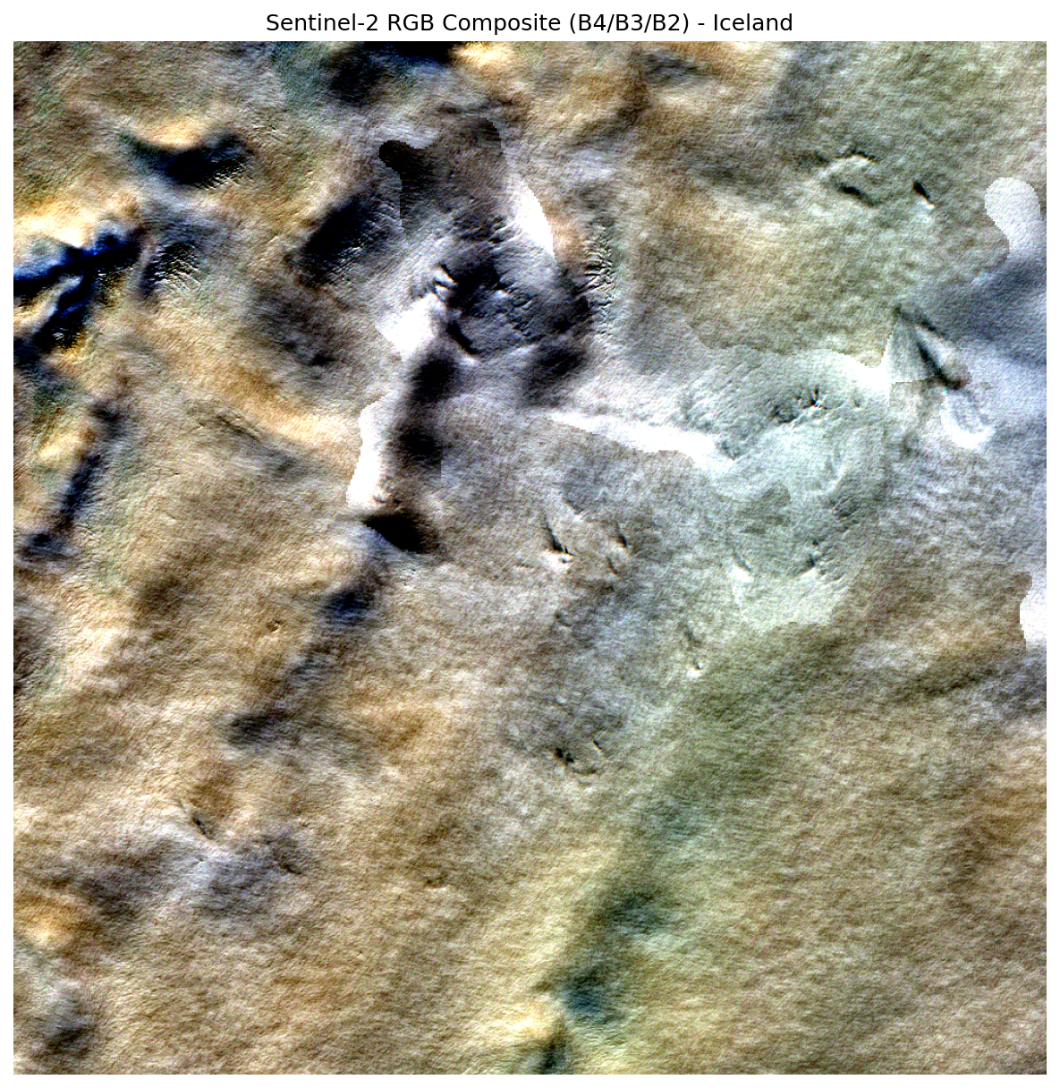
`create_rgb_composite`¶

Creates a true-color RGB composite image from Sentinel-2 10 m resolution bands (B04 Red, B03 Green, B02 Blue).

Parameters:

Parameter	Type	Required	Default	Description
`zarr_url`	string	Yes	-	URL to the SR_10m Zarr asset
`location_name`	string	No	-	Location name for the image title
`subset_size`	integer	No	`1000`	Output image dimensions (pixels)

Returns: Path to saved PNG and image metadata.

Processing Pipeline:

Stream B04, B03, B02 band data via HTTP range requests (~1-5 MB total)
Apply scale/offset: Reflectance = (DN x 0.0001) + (-0.1)
Stack bands into RGB composite
Normalize using 2-98% percentile stretch for optimal contrast
Save to outputs/rgb_composite_XXXX.png

Example:

> Create an RGB composite for the most recent image of Iceland

Executing: create_rgb_composite({
    'zarr_url': '.../.../r10m',
    'location_name': 'Iceland'
})

- Output file: outputs/rgb_composite_254.png
- Image size: 1000 x 1000 px
- Bands used: Red (B04), Green (B03), Blue (B02)

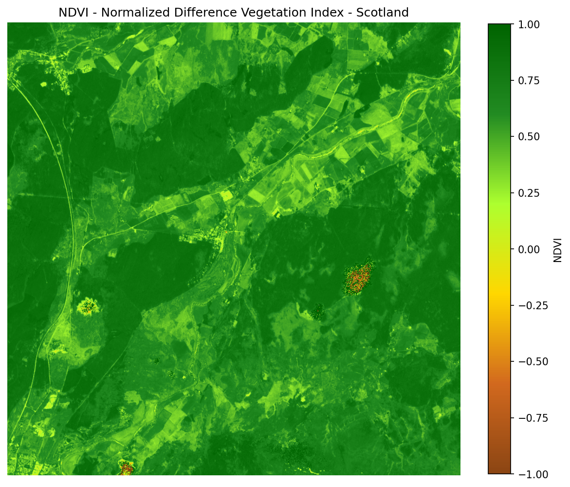
`calculate_ndvi`¶

Computes the Normalized Difference Vegetation Index (NDVI) from B08 (NIR) and B04 (Red) bands.

Formula: NDVI = (NIR - Red) / (NIR + Red)

Parameters:

Parameter	Type	Required	Default	Description
`zarr_url`	string	Yes	-	URL to the SR_10m Zarr asset
`location_name`	string	No	-	Location name for the image title
`subset_size`	integer	No	`1000`	Output image dimensions (pixels)

Returns: NDVI statistics (min, max, mean, std) and path to the saved colormap image.

NDVI Interpretation:

NDVI Range	Interpretation
< 0	Water, snow, clouds
0.0 – 0.1	Bare soil, rock, sand
0.1 – 0.3	Sparse vegetation, shrubs
0.3 – 0.6	Moderate vegetation
0.6 – 0.9	Dense, healthy vegetation

Example:

> get me recent image of scotland and its ndvi

Executing: calculate_ndvi({...})

NDVI statistics:
- Minimum: -724775
- Maximum: 161061
- Mean: -16.43
- Standard deviation: 2447.43

`get_band_statistics`¶

Retrieves statistical summaries (min, max, mean, standard deviation) for specified spectral bands from a Sentinel-2 Zarr asset.

Parameters:

Parameter	Type	Required	Default	Description
`zarr_url`	string	Yes	-	URL to the Zarr asset
`bands`	array	No	All available	List of band names to analyze

Returns: Per-band statistics dictionary.

Metadata Tools¶

These tools generate machine-readable ML metadata for Sentinel-2 scenes using the GeoCroissant standard.

`generate_croissant_metadata`¶

Generates a GeoCroissant JSON-LD metadata file for a Sentinel-2 STAC item. The output conforms to both Croissant 1.1 and GeoCroissant 1.0 and passes mlcroissant validate without errors.

Parameters:

Parameter	Type	Required	Default	Description
`item_id`	string	Yes	-	STAC item ID (e.g. `S2B_MSIL2A_20260301...`)
`location_name`	string	No	-	Location name embedded in the dataset description
`output_path`	string	No	`outputs/croissant_<id>.json`	Custom path to write the JSON-LD file

Returns: Dictionary with success, output_path, item_id, and croissant_metadata keys.

What the output includes:

Section	GeoCroissant Field	Description
Dataset identity	`@id`, `name`, `description`	Unique STAC item identifier
Spatial coverage	`spatialCoverage.geo.box`	Bounding box in WGS-84 decimal degrees
CRS	`geocr:coordinateReferenceSystem`	`EPSG:4326`
Resolution	`geocr:spatialResolution`	10 m (native Sentinel-2 resolution)
Temporal coverage	`temporalCoverage`	ISO 8601 acquisition datetime
Band configuration	`geocr:bandConfiguration`	Total bands + ordered band names
Asset distribution	`cr:FileObject`	Product Zarr URL
Band fields	`cr:Field` per band	Extraction path within the Zarr hierarchy
Citation	`citeAs`	Auto-generated BibTeX entry
Licence	`license`	CC BY 4.0

Pipeline:

flowchart LR
    A["item_id"] --> B["Fetch STAC item\nbbox, datetime, assets"]
    B --> C["Build JSON-LD context\nCroissant + GeoCroissant prefixes"]
    C --> D["Map product URL\n→ cr:FileObject"]
    D --> E["Map bands\n→ cr:Field with extract paths"]
    E --> F["Add geocr:*\nCRS, resolution, bandConfig"]
    F --> G["Save outputs/\ncroissant_<item_id>_<id>.json"]

Example:

> get me any iceland recent image geocroissant metadata

  Executing: list_recent_imagery({'location_name': 'Iceland'})
  Executing: generate_croissant_metadata({
      'item_id': 'S2B_MSIL2A_20260301T125259_N0512_R138_T27WXN_20260301T163056',
      'location_name': 'Iceland'
  })

GeoCroissant metadata saved:
  outputs/croissant_S2B_MSIL2A_20260301T125259_N0512_R138_T27WXN_20260301T163056_6007.json

Validate the output:

mlcroissant validate --jsonld=outputs/croissant_S2B_MSIL2A_20260301T125259_N0512_R138_T27WXN_20260301T163056_6007.json
# I0302 11:15:39.058333 13472 validate.py:53] Done.

Zero Errors

GeoMind's output passes mlcroissant validate with no errors or warnings on every generated file.

Direct Python Usage

You can call the tool directly without the agent:

from geomind.tools import generate_croissant_metadata

result = generate_croissant_metadata(
    item_id="S2B_MSIL2A_20260301T125259_N0512_R138_T27WXN_20260301T163056",
    location_name="Iceland",
)
print(result["output_path"])   # outputs/croissant_S2B_....json

Sentinel-2 Bands Reference¶

GeoMind works with Sentinel-2 Level-2A (surface reflectance) data.

Band	Name	Wavelength (µm)	Resolution (m)	Common Use
B01	Coastal Aerosol	0.443	60	Atmospheric correction
B02	Blue	0.490	10	RGB composites
B03	Green	0.560	10	RGB composites
B04	Red	0.665	10	RGB composites, NDVI
B05	Red Edge 1	0.704	20	Vegetation analysis
B06	Red Edge 2	0.740	20	Vegetation analysis
B07	Red Edge 3	0.783	20	Vegetation analysis
B08	NIR	0.842	10	NDVI
B8A	Narrow NIR	0.865	20	Vegetation analysis
B09	Water Vapour	0.945	60	Atmospheric correction
B11	SWIR 1	1.610	20	Moisture, snow detection
B12	SWIR 2	2.190	20	Geology, fire mapping

Tools Reference¶

Capabilities at a Glance¶

Tool Overview¶

Geocoding Tools¶

geocode_location¶

get_bbox_from_location¶

STAC Search Tools¶

list_recent_imagery¶

search_imagery¶

get_item_details¶

Processing Tools¶

create_rgb_composite¶

calculate_ndvi¶

get_band_statistics¶

Metadata Tools¶

generate_croissant_metadata¶

Sentinel-2 Bands Reference¶

`geocode_location`¶

`get_bbox_from_location`¶

`list_recent_imagery`¶

`search_imagery`¶

`get_item_details`¶

`create_rgb_composite`¶

`calculate_ndvi`¶

`get_band_statistics`¶

`generate_croissant_metadata`¶